Why Delta Compression Works - Information Theoretic Perspective
There has been quite a few papers (DeltaZip, BitDelta, FM-Delta, DeltaDQ, UltraDelta, Delta-CoME, and many more) discussing different delta compression approaches. From time to time, I get asked why delta compression works empirically and whether it can be explained theoretically. In this post, I will try to provide a brief, sloppy, and informal explanation of why delta compression works.
We are mostly interested in lossy compression, where we want to compress the model weights while still being able to use them effectively in a downstream task. LLMs or other large-scale machine learning models are hard to explain and interpret, so in this post I will focus on a very simple case: a single linear layer with the weight $W$.
If we are thinking about lossless compression, then information theory tells us that the best we can do is to compress the model weights to the entropy of the distribution of the weights. Then here comes two questions: how do we model the weight distribution, and what’s the entropy of that distribution?
Let’s take a look at the weight distribution of a single linear layer in a large language model. We will take Llama 3.2 1B Instruct model as an example:
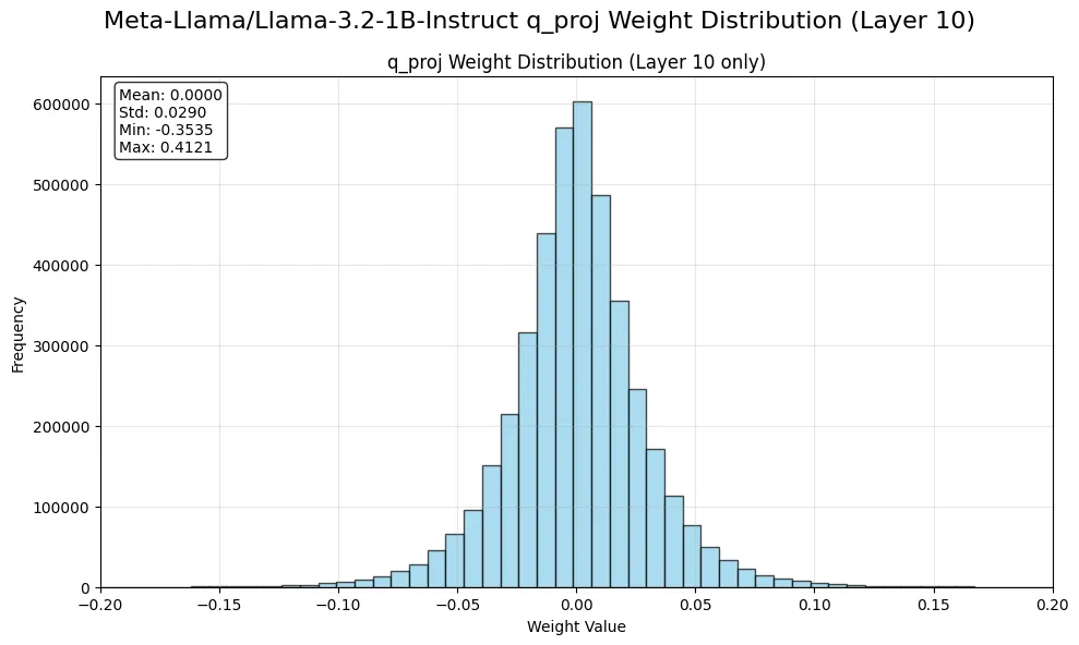
In the above figure, we can see that the weight distribution follows a Gaussian distribution with a zero mean, i.e., $W\sim \mathcal{N}(\mu, \sigma^2)$ where $\mu=0$.
Then we can compute the entropy of the weight distribution, which is given by:
$$ \begin{aligned} H(W) &= -\int p(W) \log p(W) , dW \\ &= -\mathbb{E}[\log \mathcal{N}(\mu, \sigma^2)] \\ &= -\mathbb{E}\left[\log \left( \frac{1}{\sqrt{2\pi\sigma^2}} \exp\left(-\frac{1}{2\sigma^2}(W - \mu)^2 \right) \right) \right] \\ &= \frac{1}{2} \log(2\pi \sigma^2) + \frac{1}{2\sigma^2} \mathbb{E}[(W - \mu)^2] \end{aligned} $$
Note that $\mathbb{E}[(W-\mu)^2]=\mathbb{E}[W^2]=\sigma^2$, so we have:
$$ \begin{aligned} H(W) &= \frac{1}{2}\log(2\pi \sigma^2) + \frac{1}{2} \\ &= \log(\sigma) + \frac{1}{2} + \frac{1}{2}\log(2\pi) \end{aligned} $$
This means that the entropy of the weight distribution is determined by the standard deviation $\sigma$ of the weights. The larger the standard deviation, the higher the entropy, and thus the more information we need to store. From the information theory perspective, this indicates the minimum number of bits required to represent the weights in a lossless manner.
So the first takeaway: If you have two weight matrices and you apply lossless compression, the higher the variance, the more information you need to store, and the harder it is to compress. By “the harder to compress”, it means that you will need higher bit rate.
Now that let’s consider lossy compression. In lossy compression, we extend the information theory to rate-distortion theory, which allows us to trade off between the rate (the number of bits used to represent the weights) and the distortion (the difference between the original and compressed weights).
At its core, rate-distortion theory tells us that we can compress the weights to a lower rate if we allow some distortion. The lower bound of the rate is given by the rate-distortion function $R(D)$: it’s a function between the distortion $D$ that we can tolerate and the minimum rate required to achieve that distortion.
In a simple case, we define the distortion to be the mean squared error (MSE) between the original weights and the compressed weights: $$ D = \mathbb{E}[(W -W’)^2] $$ where $W’$ is the compressed weight. We also assume that the weight distribution is Gaussian, i.e., $W \sim \mathcal{N}(\mu, \sigma^2)$ with $\mu=0$, and the values in the weight matrix are independent to each other. Then we can prove (this is a well-known theorem, you can find a proof here on page 6-7 but I will write a sketch in appendix…later) that the rate-distortion function is given by:
$$ R(D)= \begin{cases} \frac{1}{2} \log \frac{\sigma^2}{D} & 0 \le D \le \sigma^2 \\ 0 & D > \sigma^2 \end{cases} $$
We can plot the rate-distortion function as follows:
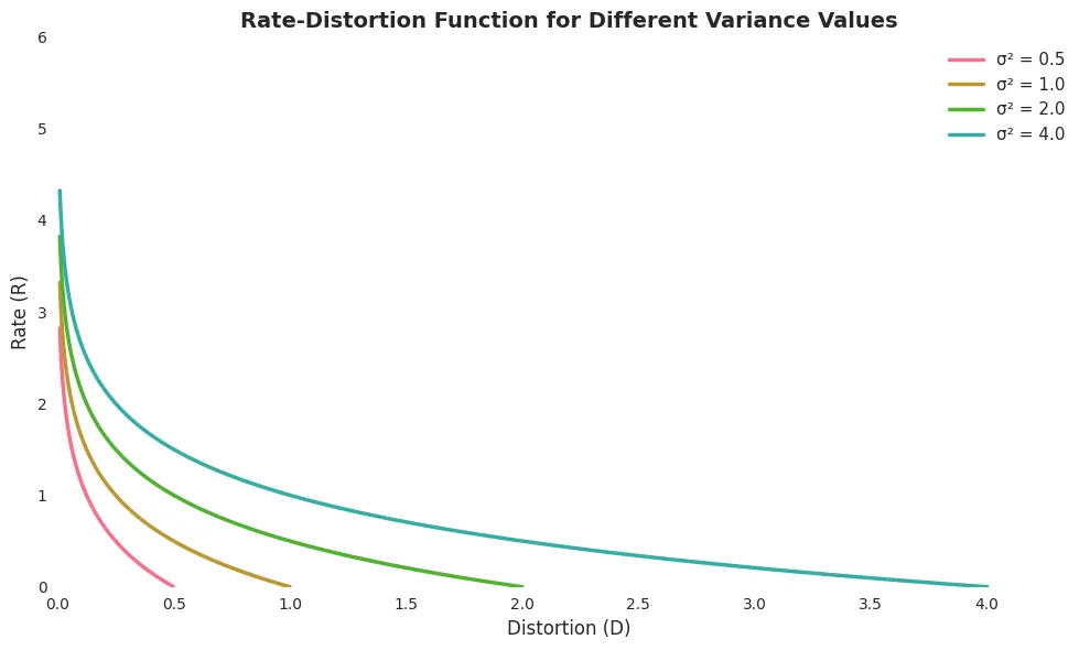
With the above rate-distortion function, we can explain it in two ways:
-
With the same level of distortion, the higher the variance of the weights, the more bits we need to represent the weights.
-
With the same bit rate, the higher the variance of the weights, the more distortion we will have.
Next we will analyze a more interesting distortion definition for us: the reconstruction error, i.e.,
$$ D’ = \mathbb{E}[(WX-W’X)^2] $$
We can write out the expansion and find that the reconstruction error is proportional to the mean squared error between the original and compressed weights, scaled by the variance of the input $X$. Hence, the rate-distortion function with the reconstruction error distortion will look similar to the one we have above. This means the above conclusions still hold.
The above analysis shows that the theoretical lower bound of bit rate required to lossily or losslessly compress the weights, is determined by the variance of the weights. However, does this still hold with the compression technique we use in practice? The answer is yes and we can verify it with empirical results. We first implement GPTQ algorithm, which is a faster approximation to the optimal brain damage (OBD) algorithm.
import mathimport timeimport torchimport torch.nn as nnimport transformersimport numpy as np
torch.backends.cuda.matmul.allow_tf32 = Falsetorch.backends.cudnn.allow_tf32 = False
DEBUG=False
def quantize(x, scale, zero, maxq):    q = torch.clamp(torch.round(x / scale) + zero, 0, maxq)    return scale * (q - zero)
class Quantizer(nn.Module):
    def __init__(self, shape=1):        super(Quantizer, self).__init__()        self.register_buffer('maxq', torch.tensor(0))        self.register_buffer('scale', torch.zeros(shape))        self.register_buffer('zero', torch.zeros(shape))
    def configure(            self,            bits, perchannel=False, sym=True,            mse=False, norm=2.4, grid=100, maxshrink=.8,            grouprows=1        ):        self.maxq = torch.tensor(2 ** bits - 1)        self.perchannel = perchannel        self.sym = sym        self.mse = mse        self.norm = norm        self.grid = grid        self.maxshrink = maxshrink        self.grouprows = grouprows
    def find_params(self, x, weight=False):        dev = x.device        self.maxq = self.maxq.to(dev)
        shape = x.shape        if self.perchannel:            if weight:                x = x.flatten(1)                if self.grouprows > 1:                    x = x.reshape((x.shape[0] // self.grouprows, -1))            else:                if len(shape) == 4:                    x = x.permute([1, 0, 2, 3])                    x = x.flatten(1)                if len(shape) == 3:                    x = x.reshape((-1, shape[-1])).t()                if len(shape) == 2:                    x = x.t()        else:            x = x.flatten().unsqueeze(0)
        tmp = torch.zeros(x.shape[0], device=dev)        xmin = torch.minimum(x.min(1)[0], tmp)        xmax = torch.maximum(x.max(1)[0], tmp)
        if self.sym:            xmax = torch.maximum(torch.abs(xmin), xmax)            tmp = xmin < 0            if torch.any(tmp):                xmin[tmp] = -xmax[tmp]        tmp = (xmin == 0) & (xmax == 0)        xmin[tmp] = -1        xmax[tmp] = +1
        self.scale = (xmax - xmin) / self.maxq        if self.sym:            self.zero = torch.full_like(self.scale, (self.maxq + 1) / 2)        else:            self.zero = torch.round(-xmin / self.scale)
        if self.mse:            best = torch.full([x.shape[0]], float('inf'), device=dev)            for i in range(int(self.maxshrink * self.grid)):                p = 1 - i / self.grid                xmin1 = p * xmin                xmax1 = p * xmax                scale1 = (xmax1 - xmin1) / self.maxq                zero1 = torch.round(-xmin1 / scale1) if not self.sym else self.zero                q = quantize(x, scale1.unsqueeze(1), zero1.unsqueeze(1), self.maxq)                q -= x                q.abs_()                q.pow_(self.norm)                err = torch.sum(q, 1)                tmp = err < best                if torch.any(tmp):                    best[tmp] = err[tmp]                    self.scale[tmp] = scale1[tmp]                    self.zero[tmp] = zero1[tmp]        if not self.perchannel:            if weight:                tmp = shape[0]            else:                tmp = shape[1] if len(shape) != 3 else shape[2]            self.scale = self.scale.repeat(tmp)            self.zero = self.zero.repeat(tmp)
        if weight:            if self.grouprows > 1:                self.scale = self.scale.unsqueeze(1).repeat(1, self.grouprows)                self.zero = self.zero.unsqueeze(1).repeat(1, self.grouprows)            shape = [-1] + [1] * (len(shape) - 1)            self.scale = self.scale.reshape(shape)            self.zero = self.zero.reshape(shape)            return        if len(shape) == 4:            self.scale = self.scale.reshape((1, -1, 1, 1))            self.zero = self.zero.reshape((1, -1, 1, 1))        if len(shape) == 3:            self.scale = self.scale.reshape((1, 1, -1))            self.zero = self.zero.reshape((1, 1, -1))        if len(shape) == 2:            self.scale = self.scale.unsqueeze(0)            self.zero = self.zero.unsqueeze(0)
    def quantize(self, x):        if self.ready():            return quantize(x, self.scale, self.zero, self.maxq)        return x
    def enabled(self):        return self.maxq > 0
    def ready(self):        return torch.all(self.scale != 0)
class SparseGPT:    def __init__(self, layer):        self.layer = layer        self.dev = self.layer.weight.device        W = layer.weight.data.clone()        if isinstance(self.layer, nn.Conv2d):            W = W.flatten(1)        if isinstance(self.layer, transformers.Conv1D):            W = W.t()        self.rows = W.shape[0]        self.columns = W.shape[1]        self.H = torch.zeros((self.columns, self.columns), device=self.dev)        self.nsamples = 0
    def add_batch(self, inp, out, blocksize=1024):        if DEBUG:            self.inp1 = inp            self.out1 = out        if len(inp.shape) == 2:            inp = inp.unsqueeze(0)        tmp = inp.shape[0]        if isinstance(self.layer, nn.Linear) or isinstance(self.layer, transformers.Conv1D):            if len(inp.shape) == 3:                inp = inp.reshape((-1, inp.shape[-1]))            inp = inp.t()        self.H *= self.nsamples / (self.nsamples + tmp)        self.nsamples += tmp        inp = math.sqrt(2 / self.nsamples) * inp.float()        self.H += inp.matmul(inp.t())
    def fasterprune(        self, sparsity, prunen=0, prunem=0, blocksize=128, percdamp=.01    ):        W = self.layer.weight.data.clone()        if isinstance(self.layer, nn.Conv2d):            W = W.flatten(1)        if isinstance(self.layer, transformers.Conv1D):            W = W.t()        W = W.float()
        if hasattr(self, 'quantizer'):            if not self.quantizer.ready():                self.quantizer.find_params(W, weight=True)
        tick = time.time()
        H = self.H        del self.H        dead = torch.diag(H) == 0        H[dead, dead] = 1        W[:, dead] = 0
        Losses = torch.zeros(self.rows, device=self.dev)
        damp = percdamp * torch.mean(torch.diag(H))        diag = torch.arange(self.columns, device=self.dev)        H[diag, diag] += damp        H = torch.linalg.cholesky(H)        H = torch.cholesky_inverse(H)        H = torch.linalg.cholesky(H, upper=True)        Hinv = H
        mask = None
        for i1 in range(0, self.columns, blocksize):            i2 = min(i1 + blocksize, self.columns)            count = i2 - i1
            W1 = W[:, i1:i2].clone()            Q1 = torch.zeros_like(W1)            Err1 = torch.zeros_like(W1)            Losses1 = torch.zeros_like(W1)            Hinv1 = Hinv[i1:i2, i1:i2]
            if prunen == 0:                if mask is not None:                    mask1 = mask[:, i1:i2]                else:                    tmp = W1 ** 2 / (torch.diag(Hinv1).reshape((1, -1))) ** 2                    thresh = torch.sort(tmp.flatten())[0][int(tmp.numel() * sparsity)]                    mask1 = tmp <= thresh            else:                mask1 = torch.zeros_like(W1) == 1
            for i in range(count):                w = W1[:, i]                d = Hinv1[i, i]
                if prunen != 0 and i % prunem == 0:                    tmp = W1[:, i:(i + prunem)] ** 2 / (torch.diag(Hinv1)[i:(i + prunem)].reshape((1, -1))) ** 2                    mask1.scatter_(1, i + torch.topk(tmp, prunen, dim=1, largest=False)[1], True)
                q = w.clone()                q[mask1[:, i]] = 0
                if hasattr(self, 'quantizer'):                    q = quantize(                        q.unsqueeze(1), self.quantizer.scale, self.quantizer.zero, self.quantizer.maxq                    ).flatten()
                Q1[:, i] = q                Losses1[:, i] = (w - q) ** 2 / d ** 2
                err1 = (w - q) / d                W1[:, i:] -= err1.unsqueeze(1).matmul(Hinv1[i, i:].unsqueeze(0))                Err1[:, i] = err1
            W[:, i1:i2] = Q1            Losses += torch.sum(Losses1, 1) / 2
            W[:, i2:] -= Err1.matmul(Hinv[i1:i2, i2:])
            if DEBUG:                self.layer.weight.data[:, :i2] = W[:, :i2]                self.layer.weight.data[:, i2:] = W[:, i2:]                print(torch.sum((self.layer(self.inp1) - self.out1) ** 2))                print(torch.sum(Losses))
        torch.cuda.synchronize()        if DEBUG:          print('time %.2f' % (time.time() - tick))          print('error', torch.sum(Losses).item())
        if isinstance(self.layer, transformers.Conv1D):            W = W.t()        self.layer.weight.data = W.reshape(self.layer.weight.shape).to(self.layer.weight.data.dtype)        if DEBUG:            print(torch.sum((self.layer(self.inp1) - self.out1) ** 2))
    def free(self):        if DEBUG:            self.inp1 = None            self.out1 = None        self.H = None        torch.cuda.empty_cache()
def compress_weight(w, x, args):  layer = nn.Linear(w.shape[1], w.shape[0])  layer.weight.data = w  y = layer(x)  compressor = SparseGPT(layer)  compressor.add_batch(x, y)  compressor.quantizer = Quantizer()  compressor.quantizer.configure(      args['wbits'], perchannel=True, sym=False, mse=False  )  compressor.fasterprune(args['sparsity'])  return compressor.layer.weight.data
With this example compression technique, we can compare the theoretical rate-distortion function with the empirical results, and here’s what we got:
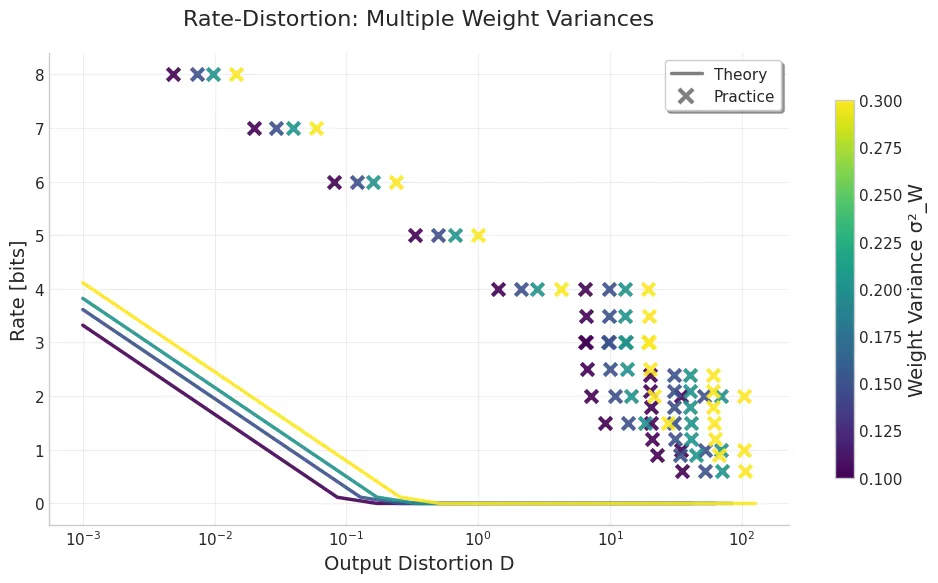
The above empirical results show that:
- GPTQ/OBD can be seen as an approximation of the optimal rate-distortion function. It does not achieve the theoretical lower bound (not even close! — suggesting better compression techniques), but it does follow the same trend as the theoretical rate-distortion function.
- With the same level of distortion, the higher the variance of the weights, the more bits we need in both practice and theory.
- With the same bit rate, the higher the variance of the weights, the more distortion we will have in both practice and theory.
Next we show empirically, the delta between fine-tuned model and the base model, exhibits smaller variance than the base model, and thus can be compressed better. We will use the Llama 3.2 1B Instruct model as an example:
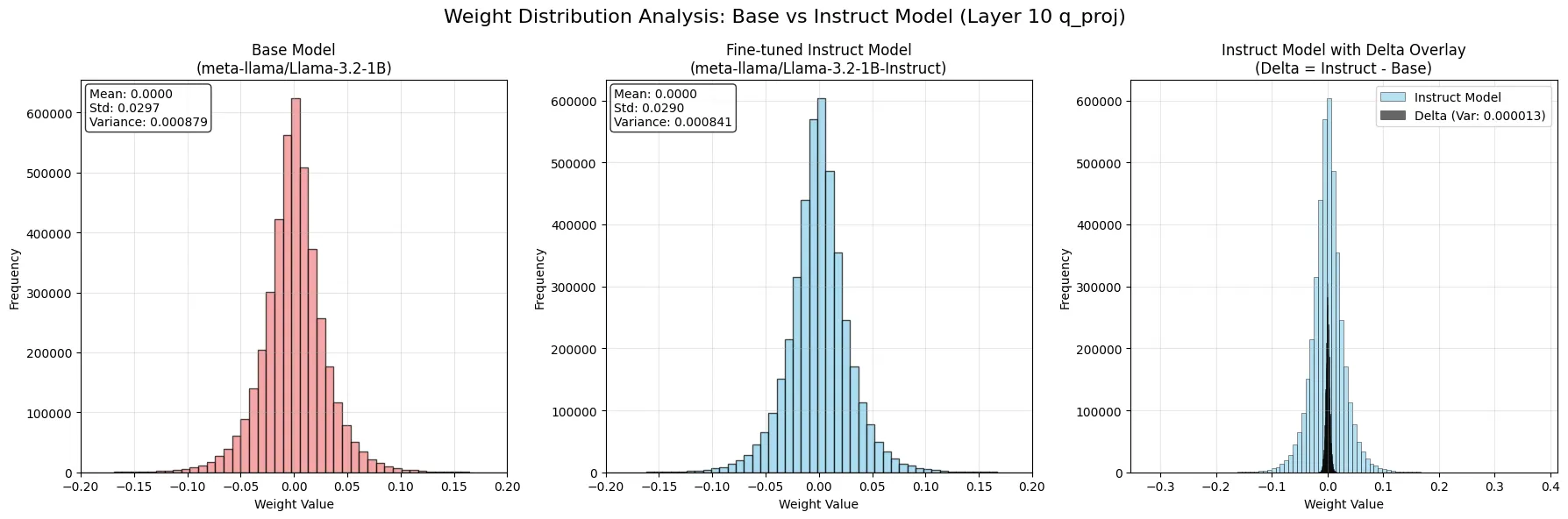
As we can see, the delta between the fine-tuned model and the base model has a smaller variance than the base model, which means that it can be compressed better. Together with the above analysis, we can conclude that delta compression works because the delta between the fine-tuned model and the base model has a smaller variance than the base model, and thus can be compressed better.
In conclusion, we showed:
- The theoretical lower bound of the bit rate required to lossily or losslessly compress the weights is determined by the variance of the weights.
- The rate-distortion function shows that with the same level of distortion, the higher the variance of the weights, the more bits we need to represent the weights.
- Empirically, OBD/GPTQ can be seen as an approximation of the optimal rate-distortion function, and it follows the same trend as the theoretical rate-distortion function.
- The delta between the fine-tuned model and the base model has a smaller variance than the base model, which means that it can be compressed better.
Cite this post (BibTeX)
@article{yao2025delta,
  title   = {Why Delta Compression Works - Information Theoretic Perspective},
  author  = {Xiaozhe Yao},
  year    = {2025},
  month   = {july},
  url     = {https://about.yao.sh/posts/why-delta-works/},
  note    = {Accessed: 2026-03-17}
}